Nozzles

Nozzles are pipes or tubes of variable cross sections. It can control the direction or characteristics of a fluid flow.

Here, tests are divided into 3 categories:

• Tank with shock.

• Injection at imposed temperature.

• Low-mach subsonic flow.

Tank with shock

It means that there is a shock in the tank which is placed before the nozzle. Initial conditions are described in Fig. 51. This test is referenced in ./libTests/referenceTestCases/euler/2D/nozzles/tankWithShock/. The corresponding uncommented line in ECOGEN.xml is:

<testCase>./libTests/referenceTestCases/euler/2D/nozzles/tankWithShock/</testCase>

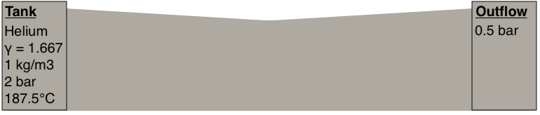
Fig. 51 Initial helium conditions before the nozzle.

Characteristic	Value
Dimension	L=1m, Øa=0.20m, Ømin=0.17m
Initial mesh structure	unstructured
Boundary conditions	inletTank, wall, outletPressure, wall
Final solution time	1.44e-2 s
Solution printing frequency	7.2e-4 s

Results are shown in Fig. 52. When helium arrives in the minimal section, there is a sonic flow. So, at the divergent section, one observes a shock wave, and then, pressure becomes stationary.

Fig. 52 Pressure evolution in the nozzle over time. Visualization using Paraview software.

The numerical solution is compared against an analytical solution in Fig. 53.

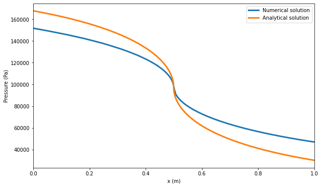
Fig. 53 Comparison between numerical and analytical pressure evolution in the nozzle over the x-direction. Visualization using Python.

The numerical solution is close to the analytical solution. Although differences exist, one should note that the code giving the analytical solution is 1D, whereas the numerical solution is 2D. Differences are therefore expected. Indeed, the 1D analytical solution cannot fully take into account the bent shock wave in the nozzle, unlike the 2D numerical solution. Also, the more the nozzle section varies, the less the analytical solution is accurate.

Pressure differences are shown in Fig. 54.

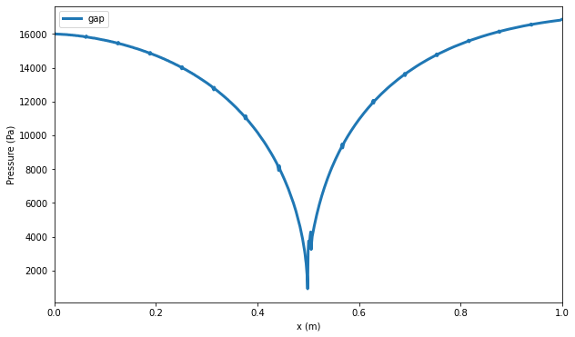
Fig. 54 Pressure difference between numerical and analytical pressures over the x-direction. Visualization using Python.

Maximum pressure differences are located at the ends of the nozzle and the minimum pressure difference is located at the minimum section.

Injection at imposed temperature

Before the nozzle, one injects air with Mach < 1. Therefore, air flow is subsonic and will cross the nozzle. Initial conditions are described on figures Fig. 55 and Fig. 56. This test is referenced in ./libTests/referenceTestCases/euler/2D/nozzles/subsonicInjection/. The corresponding uncommented line in ECOGEN.xml is:

<testCase>./libTests/referenceTestCases/euler/2D/nozzles/injectionTemp/</testCase>

Note that a variation of this test case is available where the inlet boundary is defined using a stagnation state, see test case:

<testCase>libTests/referenceTestCases/euler/2D/nozzles/injectionStagState/</testCase>

Characteristic	Value
Dimension	L=1m, Øa=0.2m, Ømin=0.17m
Initial mesh structure	unstructured
Boundary conditions	inletInjTemp, wall, outletPressure, wall
Final solution time	1s
Solution printing frequency	0.25s

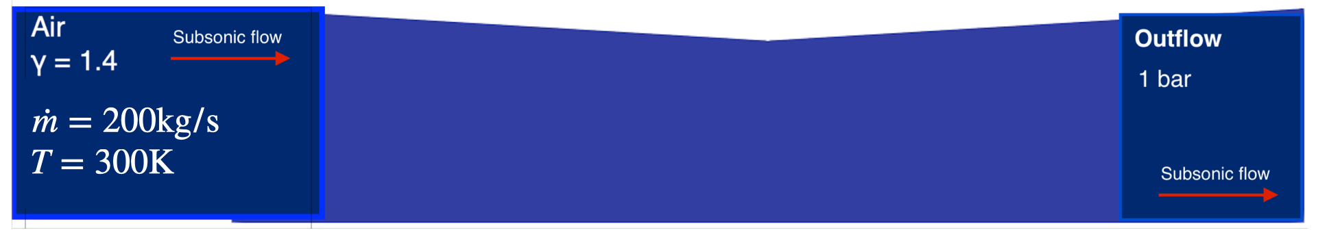
Fig. 55 Initial air conditions before the nozzle with subsonic outlet flow.

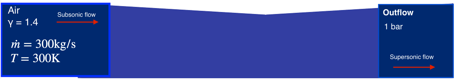
Fig. 56 Initial air conditions before the nozzle with supersonic outlet flow.

Another configuration is possible. Even thought shock wave happens in the divergent, the flow will be subsonic, otherwise, the flow will be supersonic at the exit. It depends on the critical pressure ratio.

This case is when the flow is supersonic at the exit (Fig. 57).

Fig. 57 Air velocity inside a nozzle with supersonic exit. Visualization using Paraview software.

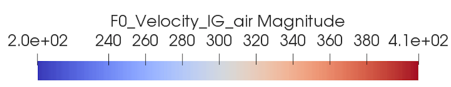
Here, the nozzle is primed at the minimal section. So, at the exit, one observes that the flow is supersonic.

This is the other case, when the flow is subsonic at the exit (Fig. 58).

Fig. 58 Air velocity inside a nozzle with subsonic exit. Visualization using Paraview software.

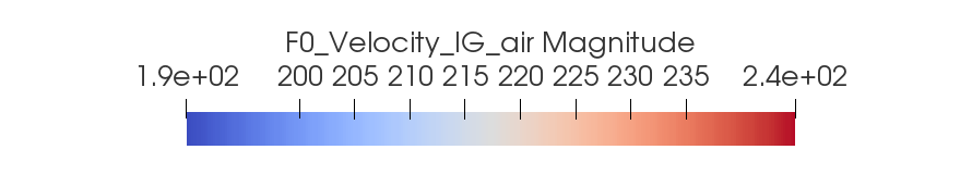
Because of a subsonic flow over the whole nozzle, it is not primed at the throat. Thus, one notices that the fluid accelerates when the section is reduced, then slows down when the section is enlarged. This is due to the conservation of the mass flow.

Low-Mach subsonic flow

In the test case provided below, a subsonic flow at really low speeds is studied:

<testCase>libTests/referenceTestCases/euler/2D/nozzles/lowMachSmoothCrossSection/</testCase>

In this configuration, liquid water flows through a smooth varying cross section nozzle. Due to the considered velocity range, the flow is nearly incompressible. To guarantee the convergence of the compressible solver to the exact solution, a low-Mach preconditionning technique is used. Section variation is modeled using a 1D scheme with smooth varying cross section. With this scheme, upper and lower boundary conditions are directly taken into consideration. For that reason, nullFlux boundary condition must be set at these boundaries (otherwise wall effects are counted twice).

Characteristic	Value
Dimension	L=1m, Øa=0.14657m, Ømin=0.06406m
Initial mesh structure	unstructured
Boundary conditions	inletInjStagState, nullFlux, outletPressure
Final solution time	2s
Solution printing frequency	0.1s

Pressure and velocity fields in the nozzle are presented below. One can notice that the low-Mach preconditionning technique (called Mref or local Mref) is required for the solution to convergence to the exact solution. Be aware that, to address a wider range of applications, local Mref is the only preconditionning method available in ECOGEN.

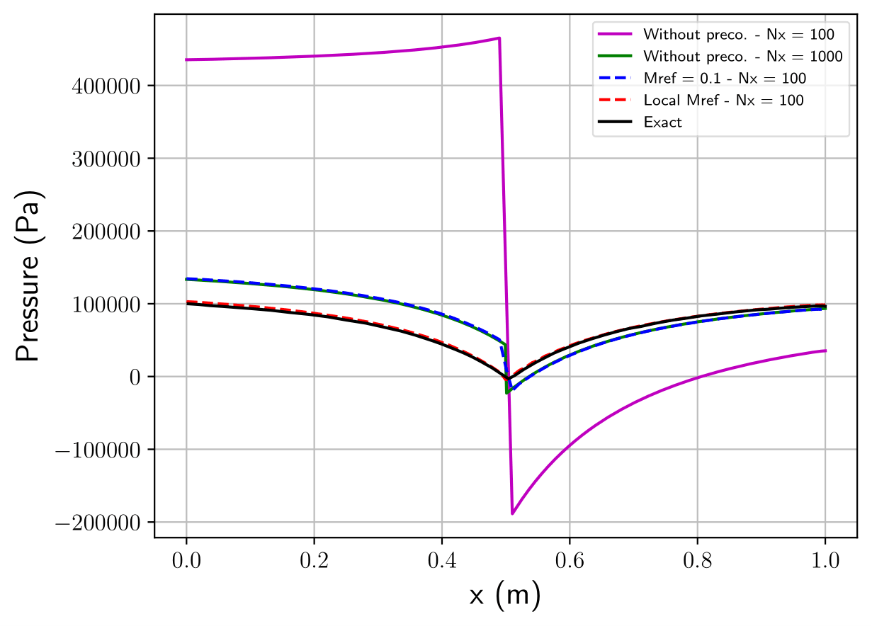
Fig. 59 Pressure field in the nozzle at steady state.

Fig. 60 Velocity field in the nozzle at steady state.

For more information on this test case and the numerical procedure, see the reference [LMNS13].