Richtmyer–Meshkov

Richtmyer–Meshkov instabilities occur when a non-regular interface between different fluids is subjected to a sudden acceleration, such as a shock wave.

Initial conditions of this test are shown in Fig. 75. Input files for this test are available in ./libTests/referenceTestCases/PUEq/2D/RichtmyerMeshkov/. The corresponding uncommented line in ECOGEN.xml is:

<testCase>./libTests/referenceTestCases/PUEq/2D/RichtmyerMeshkov/</testCase>

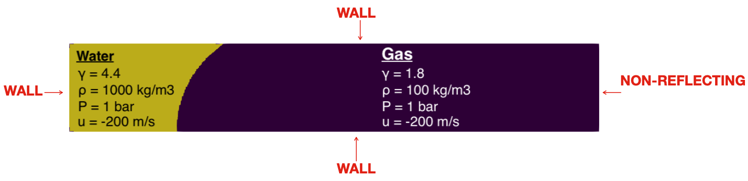
Fig. 75 Initial condition before instabilities.

The initial characteristics of the run are:

Characteristic	Value
dimension	3 m x 0.5 m
Initial mesh size	20 x 20
AMR max level	2
boundary conditions	wall ; non-reflecting
final solution time	8.6e-2 s
solution printing frequency	1.72e-3 s
precision	2nd order (VanLeer)

Results are shown in Fig. 76. Both GIFs are animations which represents on the one hand (upper half) the evolution of the mesh (AMR), that is to say its refinement for the computation of the simulation. For example, when the density variations are low or non-existent, the mesh will be as coarse as possible (within the conditions given in mesh.xml). On the contrary when the variations become significant, the mesh will become refined.

Fig. 76 Visualization of RM instabilities using Paraview software.

With the velocity u = -200m/s, the fluid impacts the left wall and a shock wave therefore propagates towards the right. This shock wave reacts with the interface and the instability takes place.

On the other hand (lower half), the second part of Fig. 76 represents the density variation (Schlieren visualization). A right-moving shock wave is created and then the Richtmyer–Meshkov instability gradually appears, with its very recognizable “mushroom” head during its non-linear phase.

One can note the distribution of computation on the CPUs (here 15) divided into different regions. The load between the regions migrates between all the CPUs during the simulation. This is shown in Fig. 77.

Fig. 77 Visualization of RM instabilities. Upper half with CPU distribution and lower half with Schlieren using Paraview software.

So, to distribute the work equally between the CPUs, highly refined regions are relatively small compared to coarse regions.