Rayleigh–Taylor

Rayleigh–Taylor instabilities occur when an irregular interface between different fluids (of different densities) is subject to a constant acceleration, like gravity. There are two types of test cases available on ECOGEN to describe Rayleigh–Taylor instabilities:

• Same dynamic viscosity,

• Same kinematic viscosity,

but only one is presented here: same kinematic viscosity.

This test case is a real two-phase test case because of the different dynamic viscosity. The proposed 2D test case is a rectangle domain with two gases of different densities. The denser of them is located at the top. Initial conditions of this test are shown in Fig. 78. Note that here a initial sinusoidal interface between the two fluids is used and is defined by:

\begin{equation*} y(x) = \cfrac{0.05}{k} \mathrm{sin} \left( \cfrac{2πx}{λ} + \cfrac{π}{2} \right) + h_m \end{equation*}

Input files for this test are available in ./libTests/referenceTestCases/PUEq/2D/RayleighTaylor/sameKinenamicViscosity/. The corresponding uncommented line in ECOGEN.xml is:

<testCase>./libTests/referenceTestCases/PUEq/2D/RayleighTaylor/sameDynamicViscosity/</testCase>

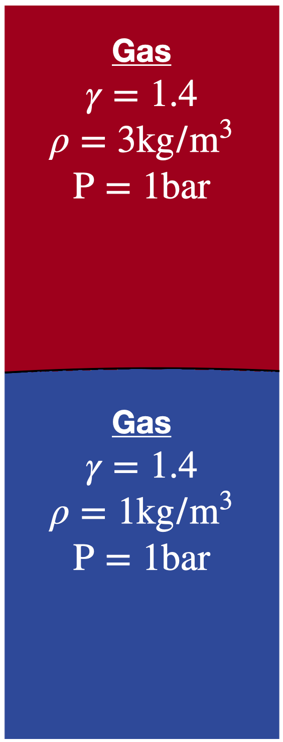
Fig. 78 Initial condition before RT instabilities. Visualization using Paraview software.

This test case is present for illustrative purposes. However, it has a strong dependency on the mesh, so it needs a refined mesh to be able to converge to the solution and thus to show correct results.

In addition, one may use Atwood number At defining the density variation with a value between 0 and 1:

\begin{equation*} At = \cfrac{\rho_h - \rho_l}{\rho_h + \rho_l} \end{equation*}

If the Atwood number tends to 1, it means there is a high-density gradient and that the phenomenon will be fast. Hence, the velocity of this instability depends on At.

The initial characteristics of the run are:

Characteristic	Value
dimension	0.1 m x 1.2 m
Initial mesh size	20 x 240
AMR max level	2
boundary conditions	wall ; symmetry
final solution time	2 s
solution printing frequency	0.1 s
precision	2nd order (VanLeer)

First of all, it is necessary to re-compile ECOGEN because it is necessary to modify a part of the GDEntireDomainWithParticularities.cpp code. Part 5 of the latter should be uncommented and “RT same dynamic viscosity” should be left commented.

After these changes, it is now necessary to compile ECOGEN again with this command:

make

or to compile and run at the same time (with 4 CPUs for example):

make && mpirun -np 4 ECOGEN

Warning

Do not forget to re-comment part 5 of GDEntireDomainWithParticularities.cpp code when recomputing another test case.

Results are shown in Fig. 79. On the right, density gradient is visualized, and on the left, mixture density is visualized with AMR. One remarks that initially the interface between the two fluids is slightly curved when the heavier fluid results in its thrust towards the lighter fluid. Then, as the instability develops its effects, irregularities (“dimples”) propagate downwards in Rayleigh–Taylor polyps. The lighter fluid expands upwards like a mushroom.

Fig. 79 RT instabilities ; mixture density (left) and density gradient (right) over time. Visualization using Paraview software.

When the density variations are low or non-existent, the mesh is as coarse as possible (within the conditions given in mesh.xml) as shown in Fig. 80. On the contrary, when the variations become significant, the mesh is refined.

Fig. 80 Magnified view of RT instabilities ; mixture density (left) and density gradient (right) over time. Visualization using Paraview software.